
Friday, July 26, 2019
Congratulations to Joe Brehm and Anna Knight for successfully defending their theses
Thursday, July 25, 2019
Edited wikipedia page of notable UNR people
I was quite astounded to find that the great ecologist William Dwight Billings was not listed on the Wikipedia page of notable UNR people. For the first time in my life I found myself editing a Wikipedia page! You can view the updated website by clicking HERE.
Dwight Billings was a leading ecologist, was known as the "father" of physiological ecology, and was a major contributor in desert and arctic ecology. In Nevada he received the prestigious Nevada medal. You can read about him by clicking HERE. Below is a partial list of his many papers which focused on our region:
Billings, W. D. (1945). The plant associations of the Carson Desert region, western Nevada. Butler University Botanical Studies, 7(1/13), 89-123.
Billings, W. D. (1949). The shadscale vegetation zone of Nevada and eastern California in relation to climate and soils. American Midland Naturalist, 87-109.
Billings, W. D. (1950). Vegetation and plant growth as affected by chemically altered rocks in the western Great Basin. Ecology, 31(1), 62-74.
Chabot, B. F., & Billings, W. D. (1972). Origins and ecology of the Sierran alpine flora and vegetation. Ecological Monographs, 42(2), 163-199.
DeLucia, E. H., Schlesinger, W. H., & Billings, W. D. (1988). Water relations and the maintenance of Sierran conifers on hydrothermally altered rock. Ecology, 69(2), 303-311.
Schlesinger, W. H., DeLucia, E. H., & Billings, W. D. (1989). Nutrient‐use efficiency of woody plants on contrasting soils in the western Great Basin, Nevada. Ecology, 70(1), 105-113.
Billings, W. D. (1994). Ecological impacts of cheatgrass and resultant fire on ecosystems in the western Great Basin. Proceedings–Ecology and Management of Annual Rangelands’.(Eds SB Monsen, SG Kitchen) pp, 22-30.
Wednesday, July 24, 2019
New ArcGIS Idea - time slider
I posted a new ArcGIS Idea "The Wayback World Imagery service is a wonderful start, but nothing beats the ease of use of Google Earth's time slider. I would love it if Esri could adopt this more streamline approach directly into ArcGIS Pro and ArcMap. We spend a lot of time using both Google Earth and ArcMap side by side. It would be wonderful if we didn't need to use both simultaneously all of the time." You can view this comment and vote on it by clicking HERE.
Thursday, July 18, 2019

Wednesday, July 17, 2019
Using GIS as a digitizer to obtain data from static graphs
There are many instances in which a person might want to obtain the actual underlying data in order to reconstruct a graph. Maybe you are doing a meta-analysis and you don't have access to the original data. Perhaps you ran the results years ago and are only now getting around to publishing. Maybe the software that you used years ago no longer exists so you can't re-run the analysis.
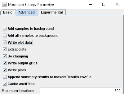
Although there are a number of digitizing software packages out there I'd suggest that for a GIS professional that GIS software might be the way to go. I recently had a case where I undertook this myself. As a quick aside it is easier to generate the data while running models. Always search your software to see if there are options for outputting the data used to build the graphs to some sort of common file type such as a CSV file. For example, Maxent software has a button that needs to checked on to output these files (see below). It is the write plot data checkbox under the Advanced tab in the older version of Maxent.
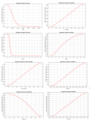
Now, back to my case study. I found myself with these terrible default graphs from Maxent (see below). No journal editor in their right mind would ever publish something like this. The font is far too small to read and there is some unnecessary titles in which the information would be in the caption in a journal manuscript. I needed something cleaner and nicer, but unfortunately I had forgotten to check the above mentioned box years ago when I did the study.
Instead I used ArcMap to take screenshots and digitize the values in order to clean up the data. Here is my workflow:
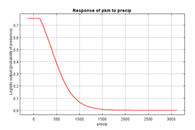
First I zoomed in and took more detailed screenshots. I used standard tools on any windows computer such as the PrtScrn button and the paint software. This resulted in a graph like the one below.
Next I imported this into ArcMap, which was as simple as dragging the file in from my desktop into an empty ArcMap instance with a data frame with an undefined projection. In ArcMap I digitized a smooth line designed to replicate the line from the Maxent software like the one below.
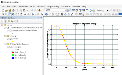
I ran a tool called Feature Vertices to Points to convert the lines to points. Feature Vertices to Points uses an Advanced license of ArcMap. If you don't have that license or want to skip the conversion I'd suggest just digitizing the points directly.
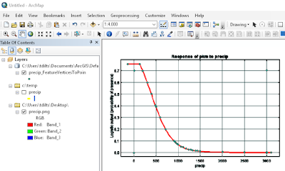
The result of the Feature Vertices to Points to conversion is shown in the image above. At this point in the process I also digitize in four additional points with known X and Y coordinates on the graph. Next I run the Add XY tool to obtain the X and Y coordinates (these are in arbitrary units). I add two additional fields called X and Y which I create as double precision. In the Field Calculator I use the following formula to calculate the X field:
(((newmax - newmin) / (oldmax - oldmin)) * ( [POINT_X] - oldmin)) + newmin
where newmax is the maximum X value of the digitized reference point as read off of the graph
where newmin is the minimum X value of the digitized reference point as read off of the graph
where oldmax is the maximum X value of the digitized reference point as calculated from the Add XY tool
where oldmin is the minimum X value of the digitized reference point as calculated from the Add XY tool
and [POINT_X] is the value from the POINT_X field in the table
The result of this and a similar formula applied to the Y value is shown below.
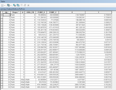
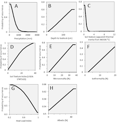
Finally I highlight the top rows skipping the four reference points and copy the data into Excel. As an alternative workflow I could have applied the field calculator formulas in Excel. Now with a little finessing in Excel (or R or whatever software you prefer) you can get some clean nice graphs like the ones below.
Although there are a number of digitizing software packages out there I'd suggest that for a GIS professional that GIS software might be the way to go. I recently had a case where I undertook this myself. As a quick aside it is easier to generate the data while running models. Always search your software to see if there are options for outputting the data used to build the graphs to some sort of common file type such as a CSV file. For example, Maxent software has a button that needs to checked on to output these files (see below). It is the write plot data checkbox under the Advanced tab in the older version of Maxent.

Now, back to my case study. I found myself with these terrible default graphs from Maxent (see below). No journal editor in their right mind would ever publish something like this. The font is far too small to read and there is some unnecessary titles in which the information would be in the caption in a journal manuscript. I needed something cleaner and nicer, but unfortunately I had forgotten to check the above mentioned box years ago when I did the study.

Instead I used ArcMap to take screenshots and digitize the values in order to clean up the data. Here is my workflow:
First I zoomed in and took more detailed screenshots. I used standard tools on any windows computer such as the PrtScrn button and the paint software. This resulted in a graph like the one below.

Next I imported this into ArcMap, which was as simple as dragging the file in from my desktop into an empty ArcMap instance with a data frame with an undefined projection. In ArcMap I digitized a smooth line designed to replicate the line from the Maxent software like the one below.

I ran a tool called Feature Vertices to Points to convert the lines to points. Feature Vertices to Points uses an Advanced license of ArcMap. If you don't have that license or want to skip the conversion I'd suggest just digitizing the points directly.

The result of the Feature Vertices to Points to conversion is shown in the image above. At this point in the process I also digitize in four additional points with known X and Y coordinates on the graph. Next I run the Add XY tool to obtain the X and Y coordinates (these are in arbitrary units). I add two additional fields called X and Y which I create as double precision. In the Field Calculator I use the following formula to calculate the X field:
(((newmax - newmin) / (oldmax - oldmin)) * ( [POINT_X] - oldmin)) + newmin
where newmax is the maximum X value of the digitized reference point as read off of the graph
where newmin is the minimum X value of the digitized reference point as read off of the graph
where oldmax is the maximum X value of the digitized reference point as calculated from the Add XY tool
where oldmin is the minimum X value of the digitized reference point as calculated from the Add XY tool
and [POINT_X] is the value from the POINT_X field in the table
The result of this and a similar formula applied to the Y value is shown below.

Finally I highlight the top rows skipping the four reference points and copy the data into Excel. As an alternative workflow I could have applied the field calculator formulas in Excel. Now with a little finessing in Excel (or R or whatever software you prefer) you can get some clean nice graphs like the ones below.

Subscribe to:
Posts (Atom)