How to get thumbnails in ArcMap

Many of us who were around pre-2010 were used to working extensively in ArcCatalog to organize and preview our data.  Some of us fondly remember the preview tab, because we could quickly get a visual of our data without the need for pulling it into a map document. ArcCatalog is still a useful tool, especially for working with metadata, buts its usefulness has been greatly diminished ever since the catalog window was added to ArcMap. Integration of the catalog window into ArcMap was a super logical and useful step, however it left me wondering if I can still preview my data without the need for loading the data into ArcMap and possibly doing time consuming things like building pyramids and raster attribute tables.  In the old days this was accomplished simply by clicking on the Preview tab as in the screenshot to the left.


I recently discovered that this is also an option in ArcMap, it just takes one extra step to get to this same preview.  In the catalog window I right-click on the dataset that I'm interested in. Then I select Item Description. I've been accustomed to using this to edit metadata. However, just recently I took the extra second to click on the Preview tab to get that old-fashioned preview that I've always loved. Like the old Preview tab in ArcCatalog this one also has a button for creating a thumbnail so that you can get an even quicker visual snapshot embedded within your metadata.

Happy GIS Day 2019!

Happy GIS Day 2019!  My celebration of GIS Day involved printing and hanging this poster.

Here is a close up of the paper below that explains what GIS Day is.

New poster "Unmanned aerial vehicles can revolutionize shrubland mapping"

I have a new poster on our lab's website titled "Unmanned aerial vehicles can revolutionize shrubland mapping". You can view it by clicking HERE.

Joe Brehm and Anna Knight theses available

The Great Basin Landscape Ecology Lab now has two new masters students - Joe Brehm and Anna Knight. Joe's thesis is titled "Cheatgrass die-off in the Great Basin: A comparison of remote sensing detection methods and identification of environments favorable to die-off" and can be downloaded by clicking HERE. Anna's thesis is titled "Watershed-scale controls on riparian vegetation distribution and dynamics: Impacts of geomorphology, climate, and disturbance" and can be downloaded by clicking HERE. Great work Anna and Joe! I'd encourage you to take a look at their theses and any papers that result from them. Anna and Joe now both reside in Moab, Utah.  Congratulations on work well done and best wishes for you in your new positions.

New ArcGIS Idea - Add options to deal with ties in cell statistics tool when selecting the majority option

I have a new idea that I've posted on ArcGIS Ideas.  If you like it please go to the website and vote it up.  You can view it by clicking HERE.

Here is the idea:

Cell statistics is an incredibly useful tool.  When using the MAJORITY option the default behavior of the tool for dealing with ties (when the two most abundant values are of equal abundance) is to create NoData.  This will often result in a map with lots of holes (NoData cells).  I would propose adding at least three options for dealing with ties.  One option would be FIRST. This would take the first value of the two tied values in the raster stack.  Another option would be LAST in which it takes the last raster of the stack with the tied value. A third option would be RANDOM. This would randomly select one of the two tied values. Finally a fourth option would be NEIGHBORHOOD. This option would expand by searching a 3x3 neighborhood and using the MAJORITY  cell in that neighborhood.  If a tie couldn't be broken using a 3x3 neighborhood then a 5x5 neighborhood would be used, etc. until all cells have a value.

Congratulations to Joe Brehm and Anna Knight for successfully defending their theses

Congratulations to Joe Brehm and Anna Knight for successfully defending their master's theses. Joe's defense presentation took place 10am, Friday July 26th, 2019 and the title of his thesis was "Cheatgrass Die-Off in the Great Basin: A Comparison of Remote Sensing Detection Methods and Identification of Environments Amenable to Die-Off". Anna's thesis presentation was Thursday, July 25, at 1 pm and the title was "Watershed-scale controls on riparian vegetation distribution and dynamics: Impacts of geomorphology, climate, and disturbance". Both presentation were very well attended and well received. You can find out more about Joe and Anna by clicking HERE and make sure to keep an eye out for their theses and scientific papers.  Great work Anna and Joe!

Edited wikipedia page of notable UNR people

I was quite astounded to find that the great ecologist William Dwight Billings was not listed on the Wikipedia page of notable UNR people. For the first time in my life I found myself editing a Wikipedia page!  You can view the updated website by clicking HERE.

Dwight Billings was a leading ecologist, was known as the "father" of physiological ecology, and was a major contributor in desert and arctic ecology. In Nevada he received the prestigious Nevada medal. You can read about him by clicking HERE. Below is a partial list of his many papers which focused on our region:

Billings, W. D. (1945). The plant associations of the Carson Desert region, western Nevada. Butler University Botanical Studies, 7(1/13), 89-123.

Billings, W. D. (1949). The shadscale vegetation zone of Nevada and eastern California in relation to climate and soils. American Midland Naturalist, 87-109.

Billings, W. D. (1950). Vegetation and plant growth as affected by chemically altered rocks in the western Great Basin. Ecology, 31(1), 62-74.

Chabot, B. F., & Billings, W. D. (1972). Origins and ecology of the Sierran alpine flora and vegetation. Ecological Monographs, 42(2), 163-199.

DeLucia, E. H., Schlesinger, W. H., & Billings, W. D. (1988). Water relations and the maintenance of Sierran conifers on hydrothermally altered rock. Ecology, 69(2), 303-311.

Schlesinger, W. H., DeLucia, E. H., & Billings, W. D. (1989). Nutrient‐use efficiency of woody plants on contrasting soils in the western Great Basin, Nevada. Ecology, 70(1), 105-113.

Billings, W. D. (1994). Ecological impacts of cheatgrass and resultant fire on ecosystems in the western Great Basin. Proceedings–Ecology and Management of Annual Rangelands’.(Eds SB Monsen, SG Kitchen) pp, 22-30.

New ArcGIS Idea - time slider

I posted a new ArcGIS Idea "The Wayback World Imagery service is a wonderful start, but nothing beats the ease of use of Google Earth's time slider.  I would love it if Esri could adopt this more streamline approach directly into ArcGIS Pro and ArcMap.  We spend a lot of time using both Google Earth and ArcMap side by side.  It would be wonderful if we didn't need to use both simultaneously all of the time." You can view this comment and vote on it by clicking HERE.

Anna Knight is defending her thesis - July 25th, 1 pm

Using GIS as a digitizer to obtain data from static graphs

There are many instances in which a person might want to obtain the actual underlying data in order to reconstruct a graph.  Maybe you are doing a meta-analysis and you don't have access to the original data.  Perhaps you ran the results years ago and are only now getting around to publishing.  Maybe the software that you used years ago no longer exists so you can't re-run the analysis.

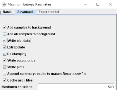
Although there are a number of digitizing software packages out there I'd suggest that for a GIS professional that GIS software might be the way to go.  I recently had a case where I undertook this myself.  As a quick aside it is easier to generate the data while running models.  Always search your software to see if there are options for outputting the data used to build the graphs to some sort of common file type such as a CSV file. For example, Maxent software has a button that needs to checked on to output these files (see below).  It is the write plot data checkbox under the Advanced tab in the older version of Maxent.



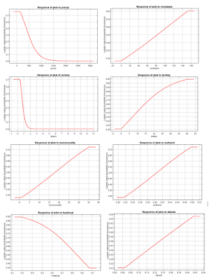
Now, back to my case study.  I found myself with these terrible default graphs from Maxent (see below).  No journal editor in their right mind would ever publish something like this.  The font is far too small to read and there is some unnecessary titles in which the information would be in the caption in a journal manuscript.  I needed something cleaner and nicer, but unfortunately I had forgotten to check the above mentioned box years ago when I did the study.



Instead I used ArcMap to take screenshots and digitize the values in order to clean up the data.  Here is my workflow:

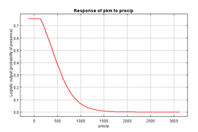
First I zoomed in and took more detailed screenshots.  I used standard tools on any windows computer such as the PrtScrn button and the paint software.  This resulted in a graph like the one below.



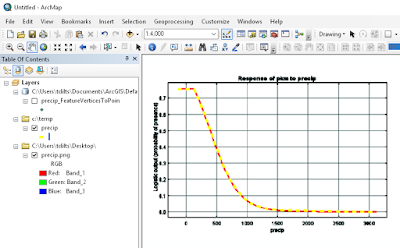
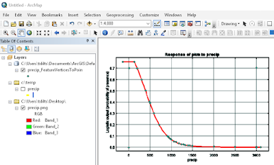
Next I imported this into ArcMap, which was as simple as dragging the file in from my desktop into an empty ArcMap instance with a data frame with an undefined projection.  In ArcMap I digitized a smooth line designed to replicate the line from the Maxent software like the one below.



I ran a tool called Feature Vertices to Points to convert the lines to points. Feature Vertices to Points uses an Advanced license of ArcMap.  If you don't have that license or want to skip the conversion I'd suggest just digitizing the points directly.


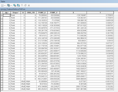
The result of the Feature Vertices to Points to conversion is shown in the image above.  At this point in the process I also digitize in four additional points with known X and Y coordinates on the graph.  Next I run the Add XY tool to obtain the X and Y coordinates (these are in arbitrary units).  I add two additional fields called X and Y which I create as double precision.  In the Field Calculator I use the following formula to calculate the X field:

(((newmax - newmin) / (oldmax - oldmin)) * ( [POINT_X] - oldmin)) + newmin

where newmax is the maximum X value of the digitized reference point as read off of the graph
where newmin is the minimum X value of the digitized reference point as read off of the graph
where oldmax is the maximum X value of the digitized reference point as calculated from the Add XY tool
where oldmin is the minimum X value of the digitized reference point as calculated from the Add XY tool
and [POINT_X] is the value from the POINT_X field in the table

The result of this and a similar formula applied to the Y value is shown below.



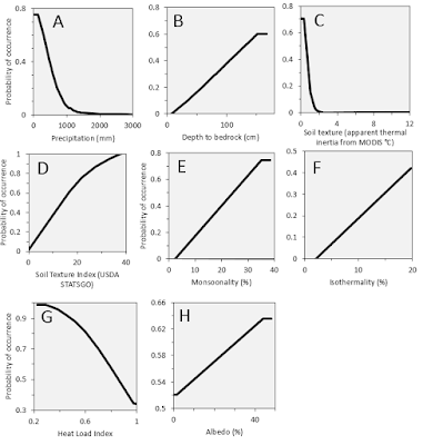
Finally I highlight the top rows skipping the four reference points and copy the data into Excel.  As an alternative workflow I could have applied the field calculator formulas in Excel.  Now with a little finessing in Excel (or R or whatever software you prefer) you can get some clean nice graphs like the ones below.

New paper - Host Plants and Climate Structure Habitat Associations of the Western Monarch Butterfly

Matt Forister, myself, and our collaborators at the Xerces Society and the USFWS have a new paper out titled "Host Plants and Climate Structure Habitat Associations of the Western Monarch Butterfly" which is published in the journal Frontiers in Ecology and Evolution. In this paper we model the habitat associations between monarch butterfly, their milkweed host plants, and a number of climatic, topographic, land use, and soil variables. We also perform habitat modeling for 13 of the most common milkweed species in the western U.S. Our study is the first large-scale habitat modeling study focused on the western population of the monarch butterfly which overwinters on the California coast and migrates inland towards the Rocky Mountains. Our paper is open access meaning that anyone can read and download it. You can go to it by clicking HERE.

To facilitate this kind of modeling we used an online citizen-science mapping tool called the Western Monarch and Milkweed Mapper. You can use the WMMM to upload your photos of monarchs and milkweeds in order to help us build better models in the future!  The WMMM also flags recent monarch sightings so that you can see when the monarchs are arriving in your area.  The WMMM also has great resources for learning how to identify the different species of milkweeds.  You can access the Western Monarch and Milkweed Mapper by clicking HERE.

Our habitat modeling work was also made possible by the tremendous amount of legwork by Madeline Steele and Joe Engler (USFWS) who completed a first version of these habitat models in 2016. Most of the variables that we used were originally compiled by Madeline, and the methods that we used followed Madeline's approach.

Finally, we should note that we have made high-resolution maps as well as details about the methodology available in the supplementary material. I would encourage you to check out these resources. For GIS users we have GeoTIFF versions of our maps available. Please contact me and I will send you a link to these files.

Citation: Dilts, T.E., Steele, M.O., Engler, J.D., Pelton, E.M., Jepsen, S.J., McKnight, S.J., Taylor, A.R., Fallon, C.E., Black, S.H., Cruz, E.E., Craver, D.R., & Forister, M.L. (2019) Host plants and climate structure habitat associations of the western monarch butterfly. Frontiers in Ecology and Evolution, 7, 188.

Excellent article in ArcUser by Jay Johnson of Washoe County

Everyone should check out the Spring 2019 issue of ArcUser.  It has a nice article by Jay Johnson of Washoe County on how they processed the recent LIDAR flight in the Reno and Sparks area.  Furthermore, the magazine cover is graced by a magnificent image of our area that is the bare earth Digital Elevation Model. You can really see the dramatic topography and almost feel the geomorphic processes taking place in our mountains and valleys!  Check out the article by clicking HERE.

New tool - Hypsometric Integral Toolbox for ArcGIS

Adriano Matos and I have put together a new tool for calculating hypsometric integral for ArcMap users. The new tool is called the Hypsometric Integral Toolbox for ArcGIS and is available by clicking HERE. You can also download this tool by clicking on our lab's tools download page HERE.

The hypsometric integral (HI) is one of the most commonly used measures that geomorphologists use to describe the shape of the Earth’s surface.  A hypsometric integral is usually calculated by plotting the cumulative height and the cumulative area under that height for individual watersheds and then taking the area under that curve to get the hypsometric integral.  In a GIS hypsometric integral is calculated by slicing watersheds into elevation bands and plotting the cumulative area for each band. Due to the iterative nature that is required for calculating hypsometric integral it tends to be one of the harder to calculate watershed variables, and thus the need for an automated tool. Although there are instructions online for how to calculate HI in ArcGIS this tool automates the processes and doesn’t require users to do their own plotting or export results to spreadsheets.

This toolbox contains two models.  Hypsometric Integral (for shapefiles only) is the main model that most users will want to run.  Hypsometric Integral (submodel) is a model that is nested within the Hypsometric Integral (for shapefiles only) model and doesn’t need to be run by itself. The tool computes the hypsometric integral for a given watershed. A new shapefile will be created representing the same watershed the user inputs, but includes a new field, "HI," representing hypsometric integral percentages.

In some instances the Hypsometric Integral (for shapefiles) will show up with a red X and won’t be useable.  The workaround for this is to open the Hypsometric Integral (for shapefiles) tool in edit mode (ModelBuilder) delete the Hypsometric Integral (submodel) and drag in your version of the Hypsometric Integral (submodel). Re-connect the following parameters: input DEM, Input Watershed, TempWorkspace, and then connect the output (HI Values for all Watersheds) to the Append tool.  Click save.

In the example map above on the left we have 19 sample watersheds from central Nevada with a Digital Elevation Model. The map above on the right shows the hypsometric integral for each of the watersheds. As you can see smaller more "canyon-like" watersheds have higher values of HI compared to the more open watersheds.

how to increase the number of unique values in ArcMap raster tables

Recently I've been encountering problems where some geoprocessing tools in ArcGIS have failed to run due to requiring too many values in the attribute table.  I came across this interesting article that I thought that I'd share.  The most interesting aspect of this is that it doesn't only pertain to viewing rasters as the summary might imply.  It is actually a critical step for getting certain tools to run.  The Combine tool in Spatial Analyst is just one tool that can benefit from increasing the number of allowed unique values.  https://support.esri.com/en/technical-article/000010117

Migrating the CWD Toolbox to the ArcGIS code sharing page

I recently fixed a bug in the Climatic Water Deficit Toolbox and moved the bug -fixed version to the ArcGIS code sharing page.

Anna Knight wins AGU Outstanding Student Presentation Award

Congratulations Anna Knight on winning Outstanding Student Presentation at the 2018 American Geophysical Union Meeting for her poster “Geomorphic and disturbance controls on vegetation dynamics in Great Basin riparian ecosystems “. Click HERE to view Anna’s poster. You can read more about AGU’s Outstanding Student Presentation by clicking HERE.

AGU is a huge conference with thousands of students attending.  Anna's award is a testament to her hard work and innovative cutting-edge techniques.  Anna is completing her master's thesis under the advisement of Dr. Peter Weisberg.  You can view her webpage by clicking HERE.