New tool - Hypsometric Integral Toolbox for ArcGIS

Adriano Matos and I have put together a new tool for calculating hypsometric integral for ArcMap users. The new tool is called the Hypsometric Integral Toolbox for ArcGIS and is available by clicking HERE. You can also download this tool by clicking on our lab's tools download page HERE.

The hypsometric integral (HI) is one of the most commonly used measures that geomorphologists use to describe the shape of the Earth’s surface.  A hypsometric integral is usually calculated by plotting the cumulative height and the cumulative area under that height for individual watersheds and then taking the area under that curve to get the hypsometric integral.  In a GIS hypsometric integral is calculated by slicing watersheds into elevation bands and plotting the cumulative area for each band. Due to the iterative nature that is required for calculating hypsometric integral it tends to be one of the harder to calculate watershed variables, and thus the need for an automated tool. Although there are instructions online for how to calculate HI in ArcGIS this tool automates the processes and doesn’t require users to do their own plotting or export results to spreadsheets.

This toolbox contains two models.  Hypsometric Integral (for shapefiles only) is the main model that most users will want to run.  Hypsometric Integral (submodel) is a model that is nested within the Hypsometric Integral (for shapefiles only) model and doesn’t need to be run by itself. The tool computes the hypsometric integral for a given watershed. A new shapefile will be created representing the same watershed the user inputs, but includes a new field, "HI," representing hypsometric integral percentages.

In some instances the Hypsometric Integral (for shapefiles) will show up with a red X and won’t be useable.  The workaround for this is to open the Hypsometric Integral (for shapefiles) tool in edit mode (ModelBuilder) delete the Hypsometric Integral (submodel) and drag in your version of the Hypsometric Integral (submodel). Re-connect the following parameters: input DEM, Input Watershed, TempWorkspace, and then connect the output (HI Values for all Watersheds) to the Append tool.  Click save.

In the example map above on the left we have 19 sample watersheds from central Nevada with a Digital Elevation Model. The map above on the right shows the hypsometric integral for each of the watersheds. As you can see smaller more "canyon-like" watersheds have higher values of HI compared to the more open watersheds.

Interesting finds in aerial photography

Every once in a while I encounter really interesting stuff when looking at digital elevation models and imagery in a GIS.  Today is one of those days. In the image below (40.8154 N 119.3856 W decimal degrees) the stream in the upper part of the image is flowing in two directions.  On the USGS topographic map it is named Rock Creek and flows to the south, but in the aerial photography it is quite evident that it also flows to the north at least some of the time.

In the image below I've zoomed in and see that a small jeep track may have caused an entire stream to shift from one basin into another (at least part of the time).

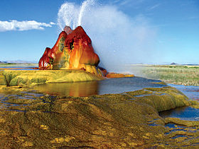
Interestingly, all of this is uphill and to the west of the cool and funky attraction known as Fly Geyser adjacent to the Black Rock Desert.

Updating 2013 NAIP Imagery in Nevada with Sun Elevation and Azimuth

NAIP imagery (National Agriculture Imagery Program of the US Department of Agriculture) constitutes a treasure trove of data that is underutilized by remote sensing analysts in my opinion. It is free, covers the entire state, and is updated regularly. So what's not to love? When it comes to image processing and classification, however, there are many challenges that people should be aware of before engaging in a major project. One challenge that I've grappled with is how to deal with differential illumination based on slope-aspect relative to the sun angle at the time of the collection. This problem can be remedied with Landsat data, because sun elevation and azimuth information is included in the metadata. The approach that we've been using in the Great Basin Landscape Ecology Lab involves creating an illumination raster (hillshade) that mimics the sun at the time of collection and then adjusts each band to its predicted brightness using linear regression.

This problem becomes more challenging with NAIP compared to Landsat, because NAIP images are flown over many months and at different times throughout the day. The result is that a single NAIP tile can have up to four different sun angles and these four regions of a single tile can have shadows pointing in four different directions. Obviously this poses a challenge to image classification.  Recently I learned that the USDA APFO now includes a seamline file for each state available for download on the Geospatial Data Gateway - https://gdg.sc.egov.usda.gov/. The approach that I'm now taking for topographic correction with NAIP involves downloading this seamline file, estimating latitude and longitude of center of each seamline polygon, and plugging this into some Excel formulas based on a NOAA spreadsheet (http://www.esrl.noaa.gov/gmd/grad/solcalc/calcdetails.html) that calculate sun elevation and azimuth.  I did this for the state of Nevada and joined the results back to the original shapefile to produce the maps below.

 

The above map shows sun elevation for NAIP flights in 2013. A higher sun elevation is good because it minimizes shadowing due to topography and vegetation. Exactly half of the area is estimated to have a sun angle between 20 and 40 degrees, with 13% below 20 degrees, and 37% greater than 40 degrees. Higher sun angles seem to be concentrated in areas north of Las Vegas and south of Tonopah. The map below shows sun azimuth. The vast majority of flights occurred when the sun was in the southeast, presumably because winds tend to be calm during the mornings.

 

The next steps involve plugging this into some tools that I've developed to topographically correct  brightness for each of the four bands and then perform classification.The caveats that come along with this analysis are as follows: 1) we assume latitude and longitude for the center of each polygon, 2) we average the beginning and end times for each polygon and plug that single time into the sun elevation and azimuth calculation, and 3) we use a 10 meter DEM because a 1 meter DEM is not available for the entire state.