Problem with Step 6 of the Climatic Water Deficit Toolbox identified and a workaround found

A while back I created the Climatic Water Deficit Toolbox for  generating climatic water deficit and actual evapotranspiration rasters. Recently I was running into a few issues with step 6 - the calculation of the soil water balance.  I was getting errors like "ERROR 010240: Could not save raster dataset ...\g_g882 with output format GRID".  It was a bit puzzling because I hadn't seen the tool creating the g_g grids before.  It turns out when the extent of the available water supply raster and the heat load raster differ then Arc creates temporary GRID files.  The remedy for this is to ensure that the available water supply and heat load rasters match exactly in extent, cell alignment, and projection.  After the two rasters were lined up the problem went away completely.

What do you do when your shapefile won't display in ArcMap?

From time to time I get e-mail questions from colleagues about what to do about the terrible and dreaded red exclamation in ArcMap.  Here are  a couple of pointers when working with shapefiles and ArcMap documents (MXD files).  First off some general advice on what to do when you get the red exclamation make:

1.  The shapefile is in the same location but the drive letters on the computer are mapped differently (e.g. Z: vs. X: vs. whatever).  If knows where it is located at it is as simple re-pathing the data.  In the Table of Contents (left panel usually) right click on the layer and go to properties.  The click the source tab followed by the set data source button.  Navigate to the file and it should update.  All other files in the same folder will be updated.  If you're using different logins then some of the locations that might be accessible to you wouldn't be to him and visa versa so that is one good reason to always save files on the network to locations that he/you can always both access.

2.  If the file was moved use the same procedure as above but navigate to the new location.

3.  Shapefiles are composed of many different files that need to be kept together.  At a minimum there is a .shp, .dbf, and .shx, but there will also be a .prj and probably a .sbn.  These files need to be kept in the same folder at all times.  If one or more of them gets moved you should move it back.

4.  As with #4 if one of those files gets deleted or corrupted you are out of luck.  Most like this isn't the case.

and some general data management tips:

1.  Always use the catalog tab in ArcMap to move, copy, or delete files.  It'll treat all of the files that compose the shapefile as a single entity.

2.  Always place your GIS files in network accessible locations and avoid the local hard drive, dektop, my documents, or temporary places that might get wiped out periodically.

3.  When editing shapefiles save frequently.  The more the better since ArcMap doesn't have an auto-save feature.

4.  Set relative paths for your ArcMap document.  File - Map Document Properties - and check 'store relative pathnames to data sources'.  There is even a setting to make this the default.  Customize - ArcMap Options - General - check 'make relative paths the default for new map documents'.

5.  Keep good mental notes where you place files and pay attention when writing outputs.  If you are ever in question go to the layer properties and view the file path or use the list by source tab in the table of contents (looks like a silver can with a yellow arrow).

6.  Practice good data management skills.  Delete old, unnecessary, duplicate, or corrupt files periodically.  Elevate final products to folder locations with really clear and memorizable paths so that you or anybody else can find your way back if necessary.  Give files really specific names that describe their purpose and avoid default names like Export_Output.  If you are going to have multiple users or multiple dates consider using suffixes with your initials and the dates to help keep track of file versioning.

Remote sensing of cheatgrass die-offs featured on YouTube

This past Tuesday Owen Baughman gave a 1 hour talk as part of the  Great Basin Landscape Conservation Cooperative's Webinar series which you can view HERE. The talk was about cheatgrass (Bromus tectorum) die-offs and whether they  present an opportunity for ecological restoration, which is the topic he studied for his Master's thesis. Although the focus of the talk was on his field experiments, which I won't describe here (better to hear it in his own words by watching the YouTube video) he did take some time to show some of the preliminary results that came about from our cheatgrass die-off remote sensing study. I'll spare you the remote sensing details and save that for when our upcoming paper comes out, but I'm proud to say that our remote sensing method for mapping cheatgrass die-offs using Landsat imagery appears to be working very well.  We developed models for 2014 using the spectral signature of known die-offs and then applied them to 2015 imagery.  Sixteen out of seventeen predicted die-offs turned out to be real die-offs when visited in the field indicating a high level of accuracy.  You can see one of the example maps for predicted die-off events in 2015 below.

Updating 2013 NAIP Imagery in Nevada with Sun Elevation and Azimuth

NAIP imagery (National Agriculture Imagery Program of the US Department of Agriculture) constitutes a treasure trove of data that is underutilized by remote sensing analysts in my opinion. It is free, covers the entire state, and is updated regularly. So what's not to love? When it comes to image processing and classification, however, there are many challenges that people should be aware of before engaging in a major project. One challenge that I've grappled with is how to deal with differential illumination based on slope-aspect relative to the sun angle at the time of the collection. This problem can be remedied with Landsat data, because sun elevation and azimuth information is included in the metadata. The approach that we've been using in the Great Basin Landscape Ecology Lab involves creating an illumination raster (hillshade) that mimics the sun at the time of collection and then adjusts each band to its predicted brightness using linear regression.

This problem becomes more challenging with NAIP compared to Landsat, because NAIP images are flown over many months and at different times throughout the day. The result is that a single NAIP tile can have up to four different sun angles and these four regions of a single tile can have shadows pointing in four different directions. Obviously this poses a challenge to image classification.  Recently I learned that the USDA APFO now includes a seamline file for each state available for download on the Geospatial Data Gateway - https://gdg.sc.egov.usda.gov/. The approach that I'm now taking for topographic correction with NAIP involves downloading this seamline file, estimating latitude and longitude of center of each seamline polygon, and plugging this into some Excel formulas based on a NOAA spreadsheet (http://www.esrl.noaa.gov/gmd/grad/solcalc/calcdetails.html) that calculate sun elevation and azimuth.  I did this for the state of Nevada and joined the results back to the original shapefile to produce the maps below.

 

The above map shows sun elevation for NAIP flights in 2013. A higher sun elevation is good because it minimizes shadowing due to topography and vegetation. Exactly half of the area is estimated to have a sun angle between 20 and 40 degrees, with 13% below 20 degrees, and 37% greater than 40 degrees. Higher sun angles seem to be concentrated in areas north of Las Vegas and south of Tonopah. The map below shows sun azimuth. The vast majority of flights occurred when the sun was in the southeast, presumably because winds tend to be calm during the mornings.

 

The next steps involve plugging this into some tools that I've developed to topographically correct  brightness for each of the four bands and then perform classification.The caveats that come along with this analysis are as follows: 1) we assume latitude and longitude for the center of each polygon, 2) we average the beginning and end times for each polygon and plug that single time into the sun elevation and azimuth calculation, and 3) we use a 10 meter DEM because a 1 meter DEM is not available for the entire state.

New paper - Functionally relevant climate variables for arid lands: using climatic water deficit modeling to predict distribution of desert shrub vegetation

I'm pleased to announce that my paper "Functionally relevant climate variables for arid lands: using climatic water deficit modeling to predict distribution of desert shrub vegetation" got accepted in the Journal of Biogeography. The paper compares two different suites of climatic variables used for modeling the distributions (climatic envelopes, niches, habitat suitability) of eighteen shrub species in the Great Basin. The first approach uses the so-called bioclimatic variables commonly used today in species distribution modeling. The latter approach uses the climatic water deficit which uses a Thornthwaite water balance model to estimate potential and actual evapotranspiration and climatic water deficit (PET minus AET). We expanded upon the work of others by deriving new variables that more fully describe the  shape of the water balance climograph. Our study found that for these shrub species there was similar model performance using the two suites of variables. However, we believe that the climatic water deficit approach may prove to be more effective in studies that predict range shifts under climate change.

The paper compliments the Climatic Water Deficit Toolbox for ArcGIS which can be found HERE. Thank you co-authors Peter Weisberg, Jeanne Chambers, and Camie Dencker as well as those who provided critical reviews.

The paper can be downloaded HERE.

Updates to the Prepare Rasters for Maxent Tool - upscaling rasters

Maxent software (http://www.cs.princeton.edu/~schapire/maxent) is frequently used for presence-only species distribution modeling. Maxent requires, however, that input ASCII raster files be aligned with one another and have the same spatial extent. This tool pre-processes raster data in preparation for Maxent modeling to ensure that all rasters have the same extent, same cell size, and aren't missing data. You can download the tool HERE.

There is a new tool that can be used to upscale data. Upscaling is useful when simple resampling is insufficient. For example, if you have a 30 meter classified vegetation map simply using the majority resample to resample to 1000 meter cell size would be insufficient because it would just tell you about the majority vegetation type present. Better would be to count the number of pixels of the vegetation type of interest within the 1000 meter cells and calculate the proportion of that vegetation type. This also solves the problem of having to treat the data as categorical in Maxent. Vegetation type would have to be treated as a categorical variable whereas proportion of X vegetation type is a continuous variable.

This example illustrates the idea of upscaling.

In the image above we have a forest/non-forest GIS layer overlaid on a coarse-resolution grid. The need for the coarse resolution grid is due to uncertainty in the location of the occurrence points and the resolution of other datasets that will be used in Maxent (e.g. the MODIS satellite products have a cell size of 250 - 1000 meters depending upon the product). The image below shows tree cover at the 1000 meter scale derived from running the Upscale Rasters for Maxent Tool. An important pre-processing step is deciding which vegetation types should be included in the model and which should be omitted. Included vegetation types should be reclassified as 1 prior to running the tool and omitted vegetation types should be reclassified as 0.

New tool - Duration of event for rasters for ArcGIS 10.1

I've got a new tool out for ArcMap that shows the duration of events. Events should be coded 1 and non-events coded 0. Each raster represents a distinct point in time (in my case I did an annual time step). You can download this new tool HERE.



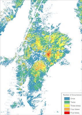
Here is an example of the tool in practice.  We've got a vegetation mortality event that can be mapped using satellite imagery. We've done this going back over twenty years at an annual time step. Each grid cell is coded either 1 or 0. The figure on the left shows the number of times that this event has occurred. We can see that in this area the event has occurred up to five times.

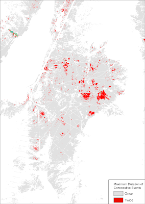
Now we run the duration tool to see if the event tends be in the same place in consecutive years.The figure below left shows that only very rarely do we see three consecutive years as having an event. Mostly we see two or even just a single consecutive events.

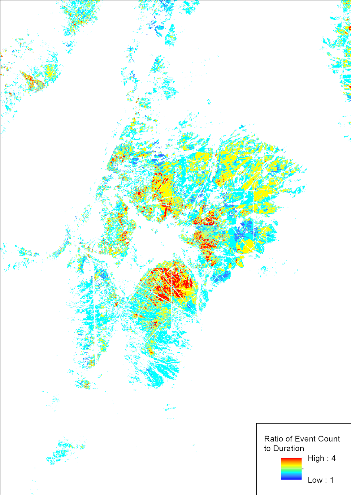
The figure below bottom shows the ratio of the count of events to the duration of events. The values range from 1 to 4 indicating that events have re-occurred in many of these areas up to four times.